Translate

Showing posts with label The Berkeley Artificial Intelligence Research Blog. Show all posts

Monday, October 5, 2020

Plan2Explore: Active Model-Building for Self-Supervised Visual Reinforcement Learning


To operate successfully in unstructured open-world environments, autonomous intelligent agents need to solve many different tasks and learn new tasks quickly. Reinforcement learning has enabled artificial agents to solve complex tasks both in simulation and real-world. However, it requires collecting large amounts of experience in the environment, and the agent learns only that particular task, much like a student memorizing a lecture without understanding. Self-supervised reinforcement learning has emerged as an alternative, where the agent only follows an intrinsic objective that is independent of any individual task, analogously to unsupervised representation learning. After experimenting with the environment without supervision, the agent builds an understanding of the environment, which enables it to adapt to specific downstream tasks more efficiently.

In this post, we explain our recent publication that develops Plan2Explore. While many recent papers on self-supervised reinforcement learning have focused on model-free agents that can only capture knowledge by remembering behaviors practiced during self-supervision, our agent learns an internal world model that lets it extrapolate beyond memorized facts by predicting what will happen as a consequence of different potential actions. The world model captures general knowledge, allowing Plan2Explore to quickly solve new tasks through planning in its own imagination. In contrast to the model-free prior work, the world model further enables the agent to explore what it expects to be novel, rather than repeating what it found novel in the past. Plan2Explore obtains state-of-the-art zero-shot and few-shot performance on continuous control benchmarks with high-dimensional input images. To make it easy to experiment with our agent, we are open-sourcing the complete source code.

How does Plan2Explore work?

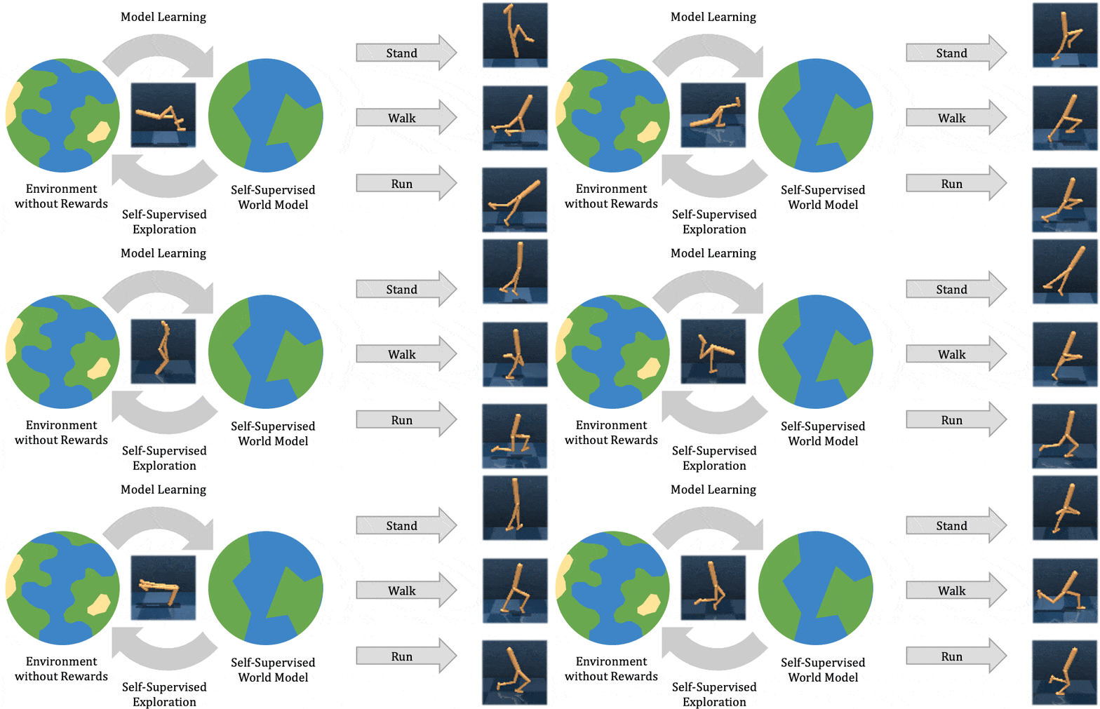
At a high level, Plan2Explore works by training a world model, exploring to maximize the information gain for the world model, and using the world model at test time to solve new tasks (see figure above). Thanks to effective exploration, the learned world model is general and captures information that can be used to solve multiple new tasks with no or few additional environment interactions. We discuss each part of the Plan2Explore algorithm individually below. We assume a basic understanding of reinforcement learning in this post.

Learning the world model

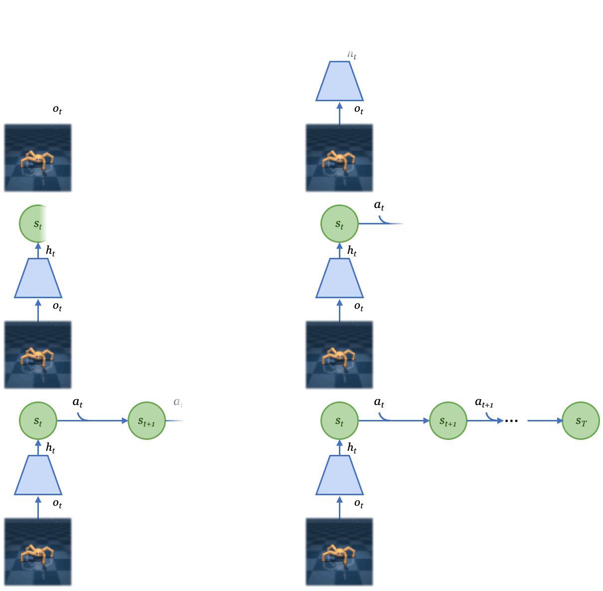
Plan2Explore learns a world model that predicts future outcomes given past observations $o_{1:t}$ and actions $a_{1:t}$. To handle high-dimensional image observations, we encode them into lower-dimensional features $h$ and use an RSSM model that predicts forward in a compact latent state-space $s$. The latent state aggregates information from past observations and is trained for future prediction, using a variational objective that reconstructs future observations. Since the latent state learns to represent the observations, during planning we can predict entirely in the latent state without decoding the images themselves. The figure below shows our latent prediction architecture.

A novelty metric for active model-building

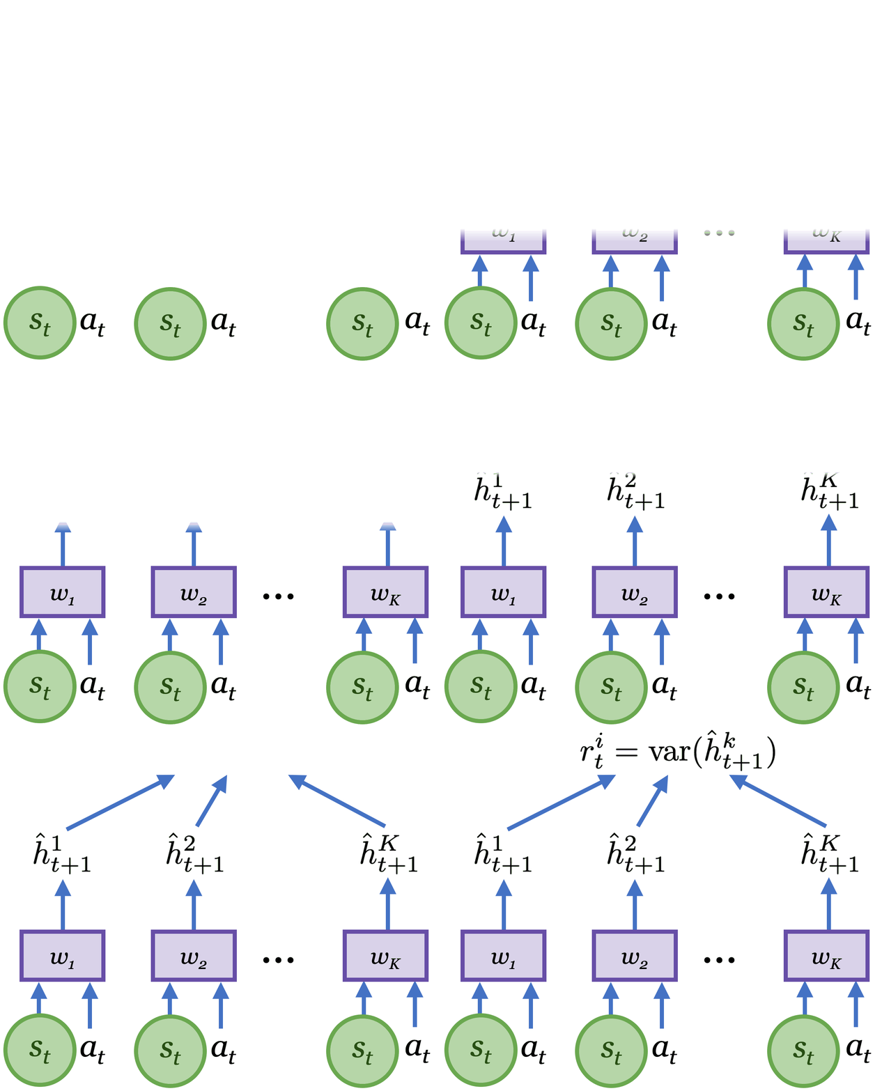
To learn an accurate and general world model we need an exploration strategy that collects new and informative data. To achieve this, Plan2Explore uses a novelty metric derived from the model itself. The novelty metric measures the expected information gained about the environment upon observing the new data. As the figure below shows, this is approximated by the disagreement of an ensemble of $K$ latent models. Intuitively, large latent disagreement reflects high model uncertainty, and obtaining the data point would reduce this uncertainty. By maximizing latent disagreement, Plan2Explore selects actions that lead to the largest information gain, therefore improving the model as quickly as possible.

Planning for future novelty

To effectively maximize novelty, we need to know which parts of the environment are still unexplored. Most prior work on self-supervised exploration used model-free methods that reinforce past behavior that resulted in novel experience. This makes these methods slow to explore: since they can only repeat exploration behavior that was successful in the past, they are unlikely to stumble onto something novel. In contrast, Plan2Explore plans for expected novelty by measuring model uncertainty of imagined future outcomes. By seeking trajectories that have the highest uncertainty, Plan2Explore explores exactly the parts of the environments that were previously unknown.

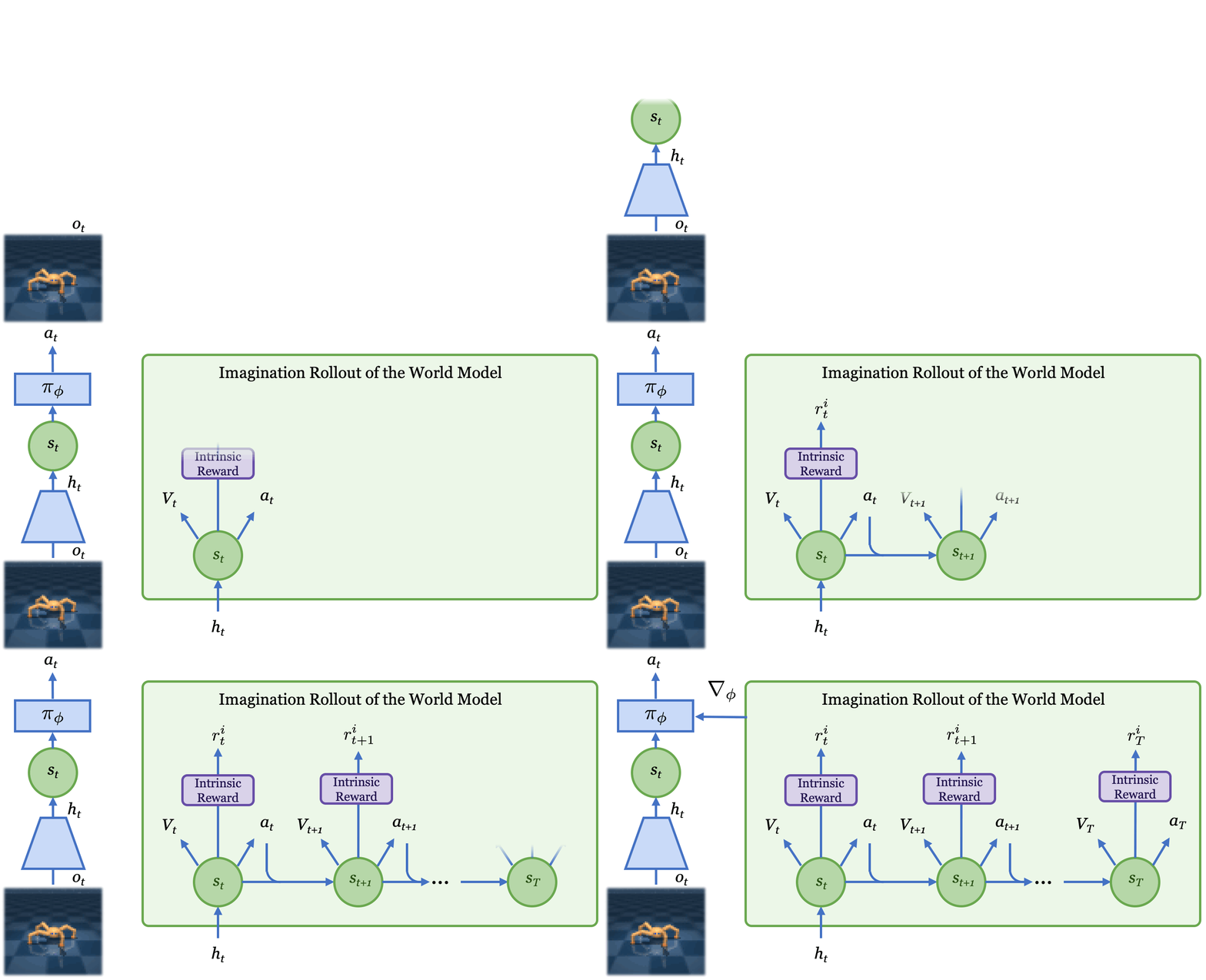
To choose actions $a$ that optimize the exploration objective, Plan2Explore leverages the learned world model as shown in the figure below. The actions are selected to maximize the expected novelty of the entire future sequence $s_{t:T}$, using imaginary rollouts of the world model to estimate the novelty. To solve this optimization problem, we use the Dreamer agent, which learns a policy $\pi_\phi$ using a value function and analytic gradients through the model. The policy is learned completely inside the imagination of the world model. During exploration, this imagination training ensures that our exploration policy is always up-to-date with the current world model and collects data that are still novel. The figure below shows the imagination training process.

Evaluation of curiosity-driven exploration behavior

We evaluate Plan2Explore on the DeepMind Control Suite, which features 20 tasks requiring different control skills, such as locomotion, balancing, and simple object manipulation. The agent only has access to image observations and no proprioceptive information. Instead of random exploration, which fails to take the agent far from the initial position, Plan2Explore leads to diverse movement strategies like jumping, running, and flipping, as shown in the figure below. Later, we will see that these are effective practice episodes that enable the agent to quickly learn to solve various continuous control tasks.


Evaluation of downstream task performance

Once an accurate and general world model is learned, we test Plan2Explore on previously unseen tasks. Given a task specified with a reward function, we use the model to optimize a policy for that task. Similar to our exploration procedure, we optimize a new value function and a new policy head for the downstream task. This optimization uses only predictions imagined by the model, enabling Plan2Explore to solve new downstream tasks in a zero-shot manner without any additional interaction with the world.

The following plot shows the performance of Plan2Explore on tasks from DM Control Suite. Before 1 million environment steps, the agent doesn’t know the task and simply explores. The agent solves the task as soon as it is provided at 1 million steps, and keeps improving fast in a few-shot regime after that.
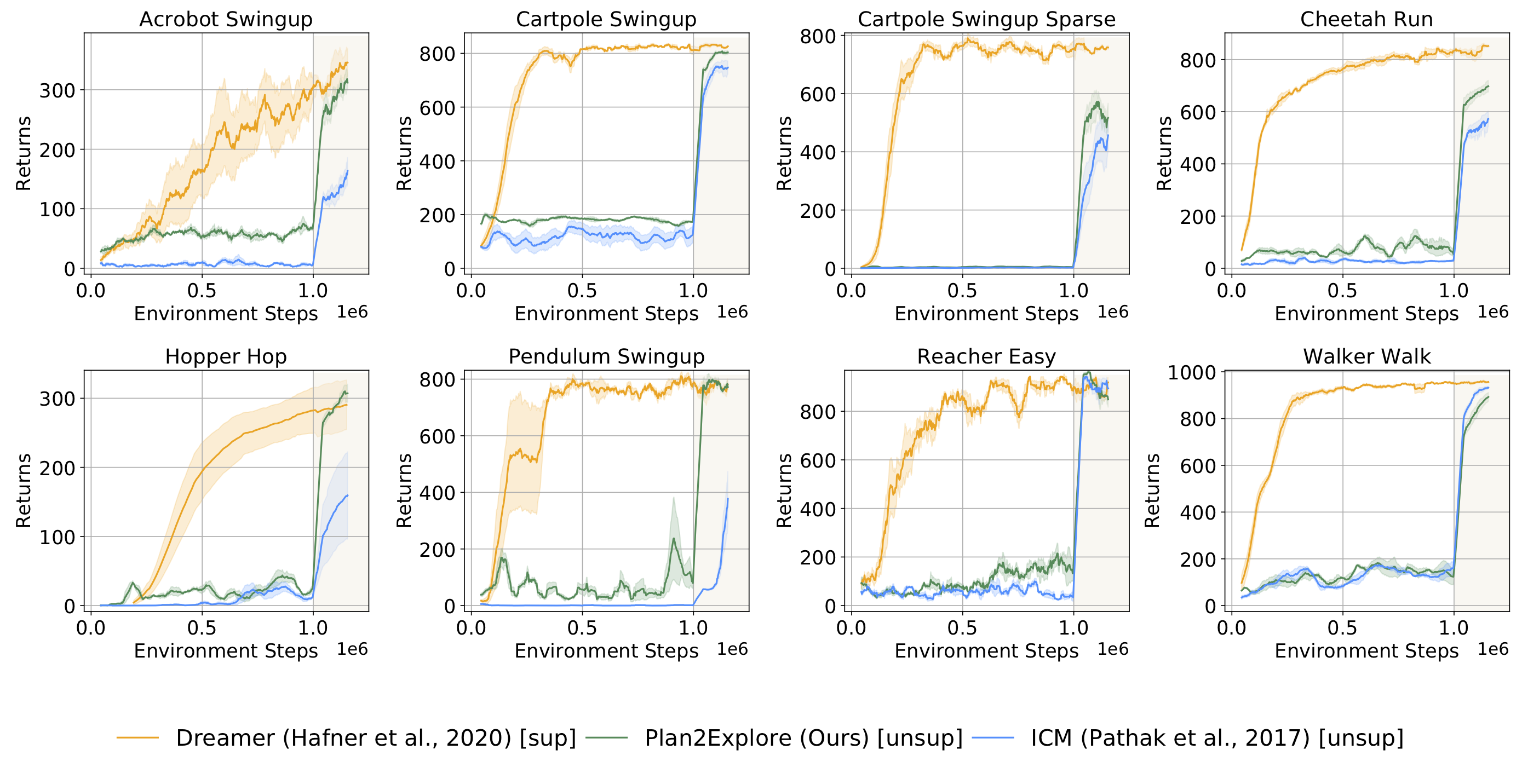

Plan2Explore () is able to solve most of the tasks we benchmarked. Since prior work on self-supervised reinforcement learning used model-free agents that are not able to adapt in a zero-shot manner (ICM, ), or did not use image observations, we compare by adapting this prior work to our model-based Plan2Explore setup. Our latent disagreement objective outperforms other previously proposed objectives. More interestingly, the final performance of Plan2Explore is comparable to the state-of-the-art oracle agent that requires task rewards throughout training (). In our paper, we further report performance of Plan2Explore in the zero-shot setting where the agent needs to solve the task before any task-oriented practice.

Future directions

Plan2Explore demonstrates that effective behavior can be learned through self-supervised exploration only. This opens multiple avenues for future research:

  • First, to apply self-supervised RL to a variety of settings, future work will investigate different ways of specifying the task and deriving behavior from the world model. For example, the task could be specified with a demonstration, description of the desired goal state, or communicated to the agent in natural language.

  • Second, while Plan2Explore is completely self-supervised, in many cases a weak supervision signal is available, such as in hard exploration games, human-in-the-loop learning, or real life. In such a semi-supervised setting, it is interesting to investigate how weak supervision can be used to steer exploration towards the relevant parts of the environment.

  • Finally, Plan2Explore has the potential to improve the data efficiency of real-world robotic systems, where exploration is costly and time-consuming, and the final task is often unknown in advance.

By designing a scalable way of planning to explore in unstructured environments with visual observations, Plan2Explore provides an important step toward self-supervised intelligent machines.


We would like to thank Georgios Georgakis and the editors of CMU and BAIR blogs for the useful feedback.

This post is based on the following paper:

  • Planning to Explore via Self-Supervised World Models
    Ramanan Sekar*, Oleh Rybkin*, Kostas Daniilidis, Pieter Abbeel, Danijar Hafner, Deepak Pathak
    Thirty-seventh International Conference Machine Learning (ICML), 2020.
    arXiv, Project Website


from The Berkeley Artificial Intelligence Research Blog https://ift.tt/30Bm4Hc
via A.I .Kung Fu

Wednesday, September 9, 2020

AWAC: Accelerating Online Reinforcement Learning with Offline Datasets


Our method learns complex behaviors by training offline from prior datasets (expert demonstrations, data from previous experiments, or random exploration data) and then fine-tuning quickly with online interaction.

Robots trained with reinforcement learning (RL) have the potential to be used across a huge variety of challenging real world problems. To apply RL to a new problem, you typically set up the environment, define a reward function, and train the robot to solve the task by allowing it to explore the new environment from scratch. While this may eventually work, these “online” RL methods are data hungry and repeating this data inefficient process for every new problem makes it difficult to apply online RL to real world robotics problems. What if instead of repeating the data collection and learning process from scratch every time, we were able to reuse data across multiple problems or experiments? By doing so, we could greatly reduce the burden of data collection with every new problem that is encountered. With hundreds to thousands of robot experiments being constantly run, it is of crucial importance to devise an RL paradigm that can effectively use the large amount of already available data while still continuing to improve behavior on new tasks.

The first step towards moving RL towards a data driven paradigm is to consider the general idea of offline (batch) RL. Offline RL considers the problem of learning optimal policies from arbitrary off-policy data, without any further exploration. This is able to eliminate the data collection problem in RL, and incorporate data from arbitrary sources including other robots or teleoperation. However, depending on the quality of available data and the problem being tackled, we will often need to augment offline training with targeted online improvement. This problem setting actually has unique challenges of its own. In this blog post, we discuss how we can move RL from training from scratch with every new problem to a paradigm which is able to reuse prior data effectively, with some offline training followed by online finetuning.


Figure 1: The problem of accelerating online RL with offline datasets. In (1), the robot learns a policy entirely from an offline dataset. In (2), the robot gets to interact with the world and collect on-policy samples to improve the policy beyond what it could learn offline.

Challenges in Offline RL with Online Fine-tuning

We analyze the challenges in the problem of learning from offline data and subsequent fine-tuning, using the standard benchmark HalfCheetah locomotion task. The following experiments are conducted with a prior dataset consisting of 15 demonstrations from an expert policy and 100 suboptimal trajectories sampled from a behavioral clone of these demonstrations.


Figure 2: On-policy methods are slow to learn compared to off-policy methods, due to the ability of off-policy methods to “stitch" good trajectories together, illustrated on the left. Right: in practice, we see slow online improvement using on-policy methods.

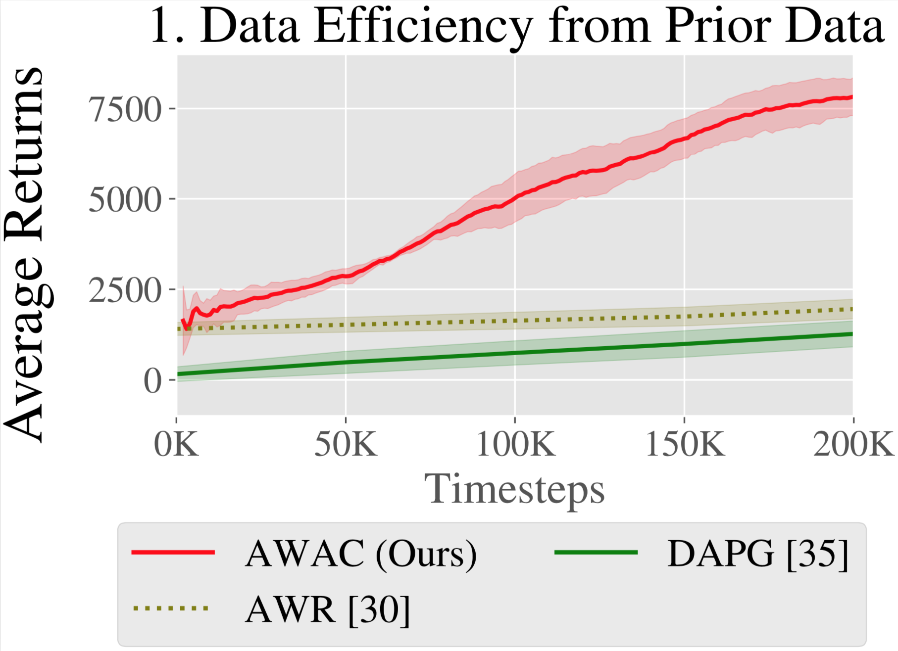
1. Data Efficiency

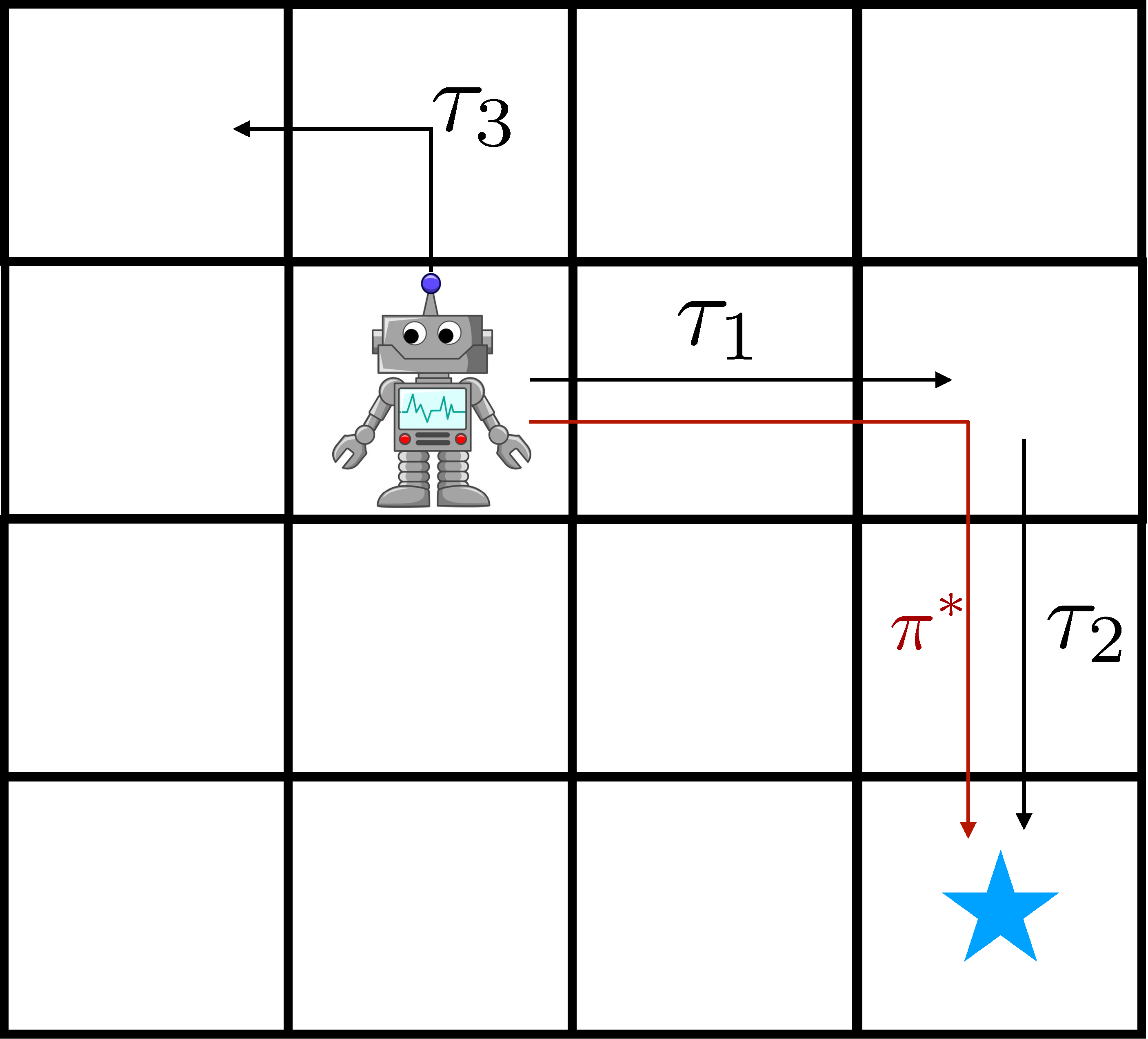
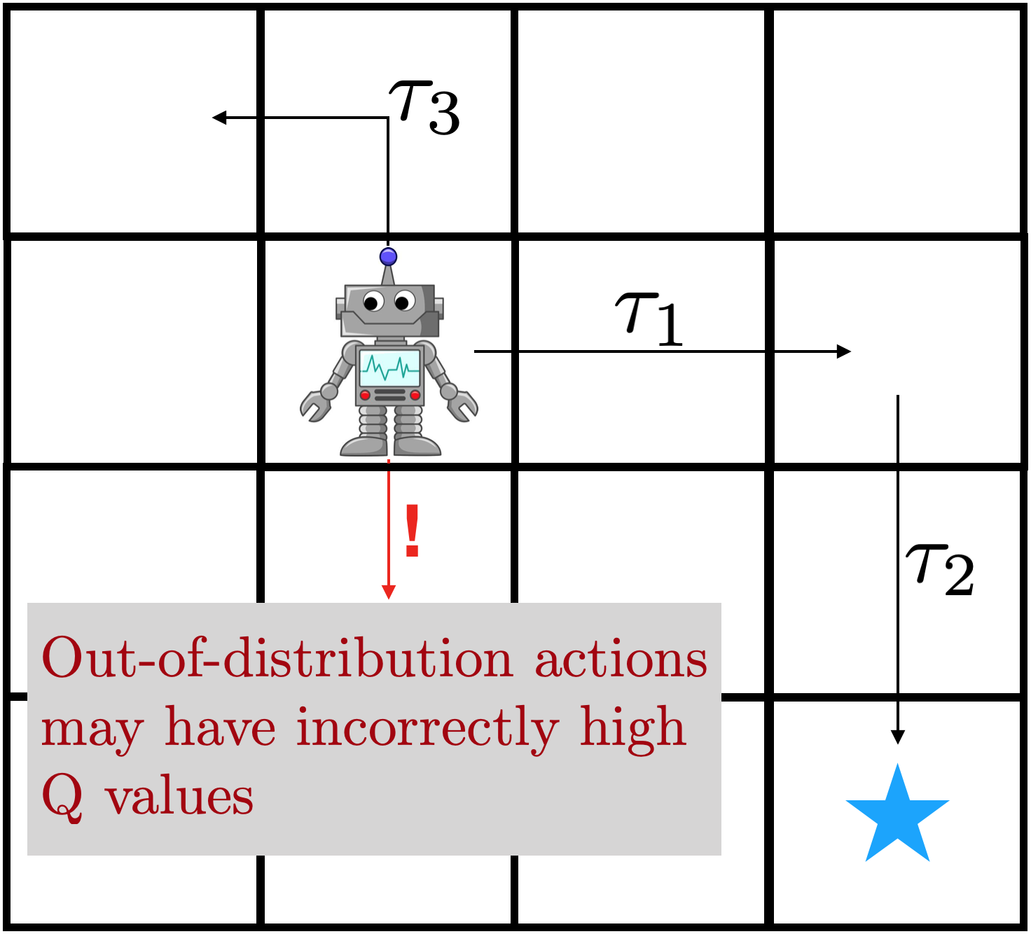
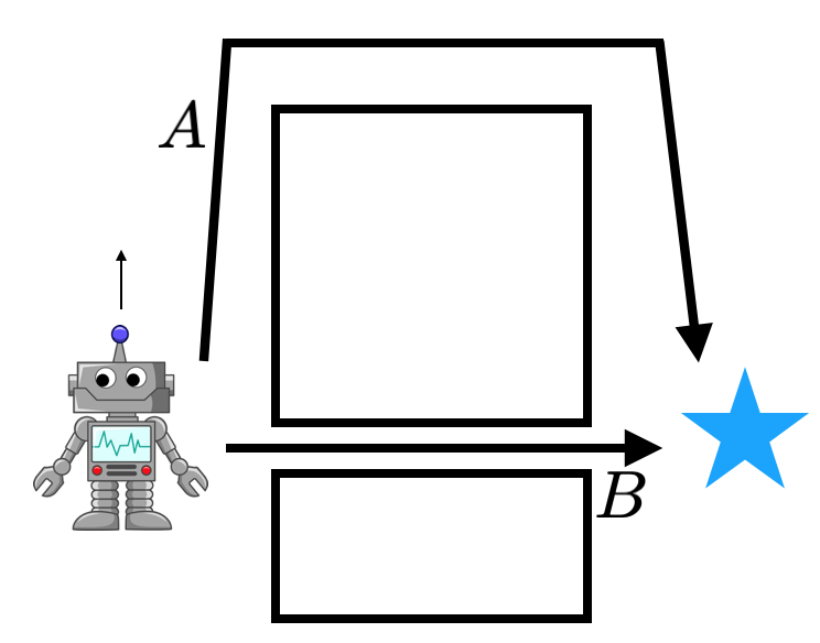
A simple way to utilize prior data such as demonstrations for RL is to pre-train a policy with imitation learning, and fine-tune with on-policy RL algorithms such as AWR or DAPG. This has two drawbacks. First, the prior data may not be optimal so imitation learning may be ineffective. Second, on-policy fine-tuning is data inefficient as it does not reuse the prior data in the RL stage. For real-world robotics, data efficiency is vital. Consider the robot on the right, trying to reach the goal state with prior trajectory $\tau_1$ and $\tau_2$. On-policy methods cannot effectively use this data, but off-policy algorithms that do dynamic programming can, by effectively “stitching” $\tau_1$ and $\tau_2$ together with the use of a value function or model. This effect can be seen in the learning curves in Figure 2, where on-policy methods are an order of magnitude slower than off-policy actor-critic methods.


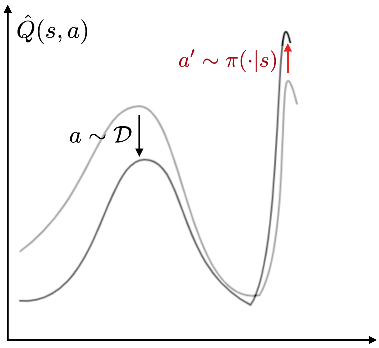
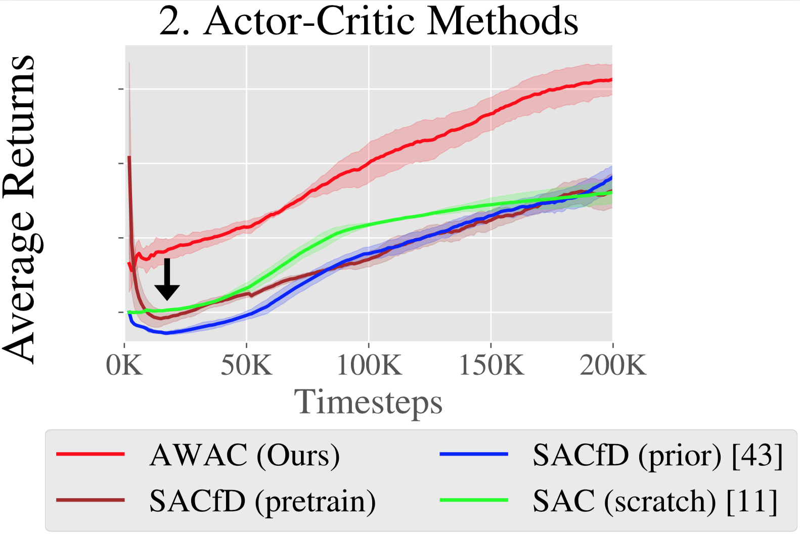
Figure 3: Bootstrapping error is an issue when using off-policy RL for offline training. Left: an erroneous Q value far away from the data is exploited by the policy, resulting in a poor update of the Q function. Middle: as a result, the robot may take actions that are out of distribution. Right: bootstrap error causes poor offline pretraining when using SAC and its variants.

2. Bootstrapping Error

Actor-critic methods can in principle learn efficiently from off-policy data by estimating a value estimate $V(s)$ or action-value estimate $Q(s, a)$ of future returns by Bellman bootstrapping. However, when standard off-policy actor-critic methods are applied to our problem (we use SAC), they perform poorly, as shown in Figure 3: despite having a prior dataset in the replay buffer, these algorithms do not benefit significantly from offline training (as seen by the comparison between the SAC(scratch) and SACfD(prior) lines in Figure 3). Moreover, even if the policy is pre-trained by behavior cloning (“SACfD (pretrain)”) we still observe an initial decrease in performance.

This challenge can be attributed to off-policy bootstrapping error accumulation. During training, the Q estimates will not be fully accurate, particularly in extrapolating actions that are not present in the data. The policy update exploits overestimated Q values, making the estimated Q values worse. The issue is illustrated in the figure: incorrect Q values result in an incorrect update to the target Q values, which may result in the robot taking a poor action.

3. Non-stationary Behavior Models

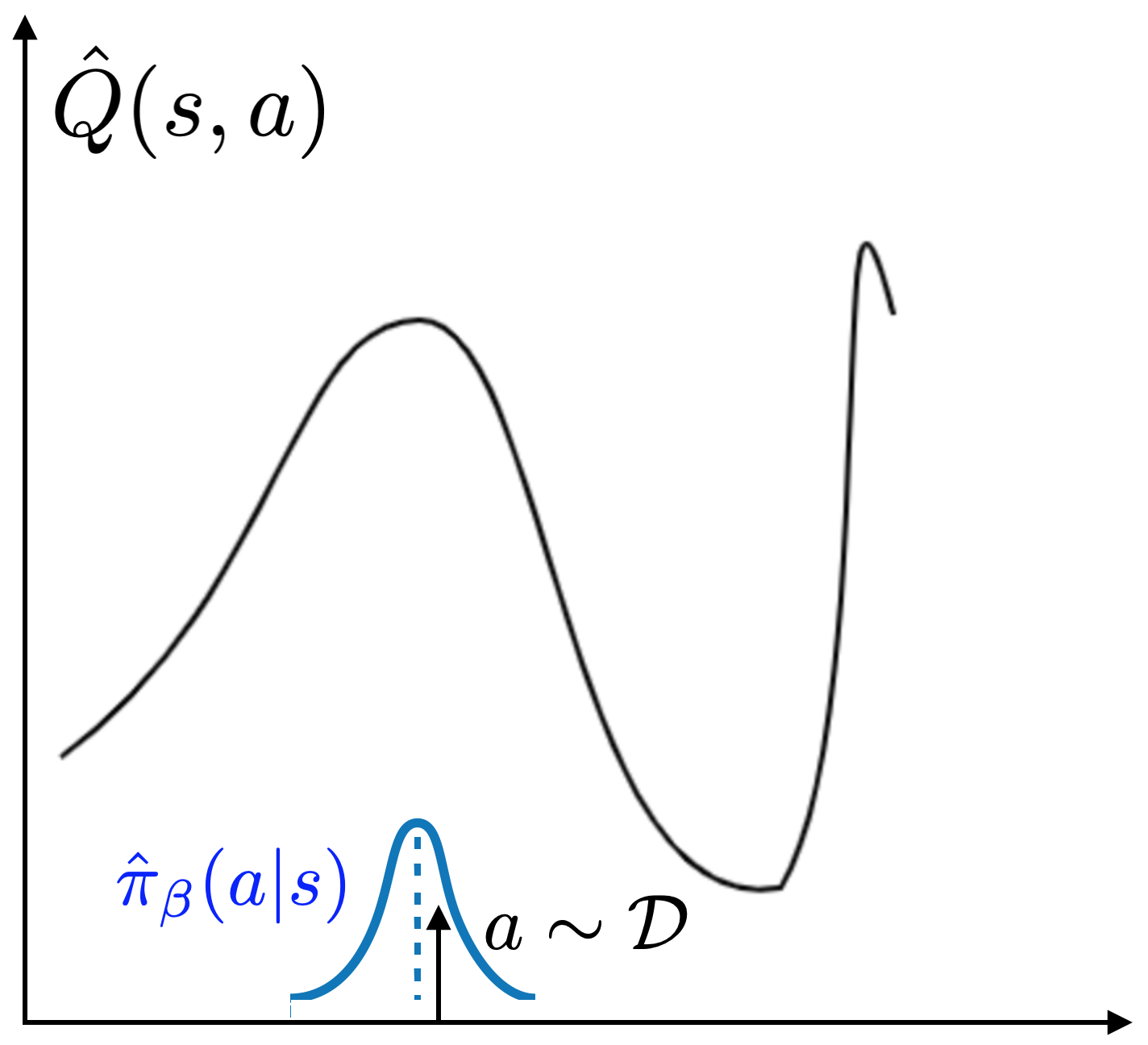
Prior offline RL algorithms such as BCQ, BEAR, and BRAC propose to address the bootstrapping issue by preventing the policy from straying too far from the data. The key idea is to prevent bootstrapping error by constraining the policy $\pi$ close to the “behavior policy” $\pi_\beta$: the actions that are present in the replay buffer. The idea is illustrated in the figure below: by sampling actions from $\pi_\beta$, you avoid exploiting incorrect Q values far away from the data distribution.

However, $\pi_\beta$ is typically not known, especially for offline data, and must be estimated from the data itself. Many offline RL algorithms (BEAR, BCQ, ABM) explicitly fit a parametric model to samples from the replay buffer for the distribution $\pi_\beta$. After forming an estimate $\hat{\pi}_\beta$, prior methods implement the policy constraint in various ways, including penalties on the policy update (BEAR, BRAC) or architecture choices for sampling actions for policy training (BCQ, ABM).

While offline RL algorithms with constraints perform well offline, they struggle to improve with fine-tuning, as shown in the third plot in Figure 1. We see that the purely offline RL performance (at “0K” in Fig.1) is much better than SAC. However, with additional iterations of online fine-tuning, the performance increases very slowly (as seen from the slope of the BEAR curve in Fig 1). What causes this phenomenon?

The issue is in fitting an accurate behavior model as data is collected online during fine-tuning. In the offline setting, behavior models must only be trained once, but in the online setting, the behavior model must be updated online to track incoming data. Training density models online (in the “streaming” setting) is a challenging research problem, made more difficult by a potentially complex multi-modal behavior distribution induced by the mixture of online and offline data. In order to address our problem setting, we require an off-policy RL algorithm that constrains the policy to prevent offline instability and error accumulation, but is not so conservative that it prevents online fine-tuning due to imperfect behavior modeling. Our proposed algorithm, which we discuss in the next section, accomplishes this by employing an implicit constraint, which does not require any explicit modeling of the behavior policy.


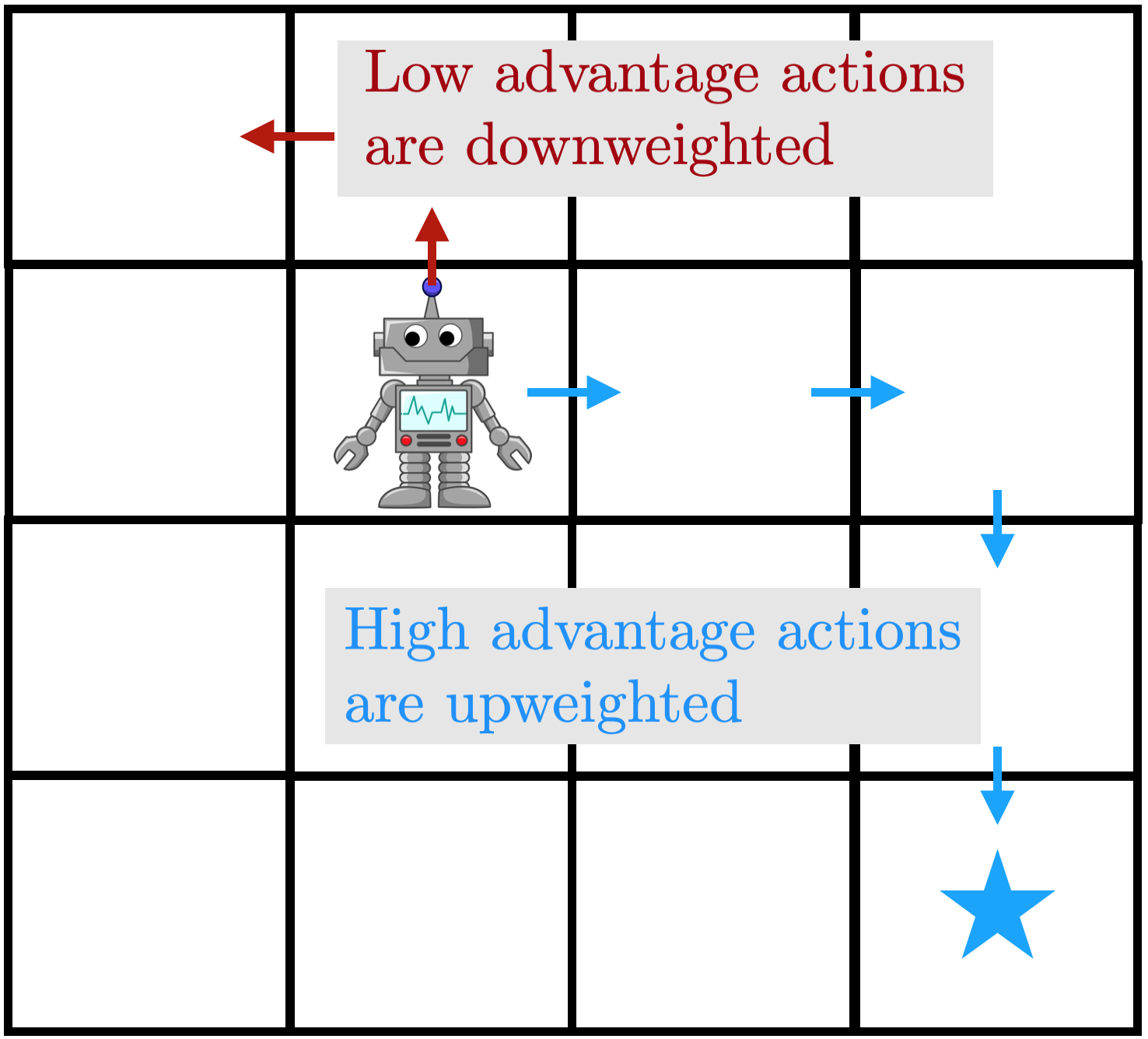
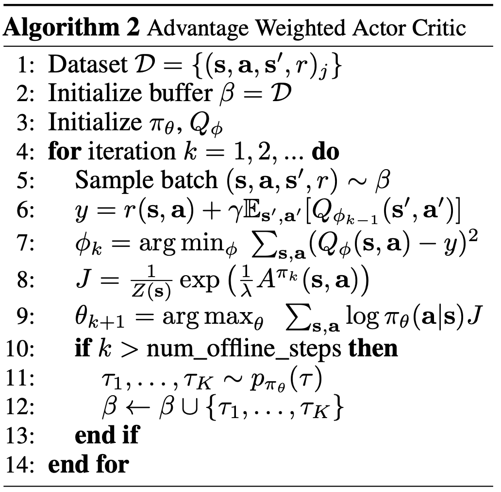
Figure 4: an illustration of AWAC. High-advantage transitions are regressed on with high weight, while low advantage transitions have low weight. Right: algorithm pseudocode.

Advantage Weighted Actor Critic

In order to avoid these issues, we propose an extremely simple algorithm - advantage weighted actor critic (AWAC). AWAC avoids the pitfalls in the previous section with careful design decisions. First, for data efficiency, the algorithm trains a critic that is trained with dynamic programming. Now, how can we use this critic for offline training while avoiding the bootstrapping problem, while also avoiding modeling the data distribution, which may be unstable? For avoiding bootstrapping error, we optimize the following problem:

We can compute the optimal solution for this equation and project our policy onto it, which results in the following actor update:

This results in an intuitive actor update, that is also very effective in practice. The update resembles weighted behavior cloning; if the Q function was uninformative, it reduces to behavior cloning the replay buffer. But with a well-formed Q estimate, we weight the policy towards only good actions. An illustration is given in the figure above: the agent regresses onto high-advantage actions with a large weight, while almost ignoring low-advantage actions. Please see the paper for an expanded derivation and implementation details.

Experiments

So how well does this actually do at addressing our concerns from earlier? In our experiments, we show that we can learn difficult, high-dimensional, sparse reward dexterous manipulation problems from human demonstrations and off-policy data. We then evaluate our method with suboptimal prior data generated by a random controller. Results on standard MuJoCo benchmark environments (HalfCheetah, Walker, and Ant) are also included in the paper.

Dexterous Manipulation


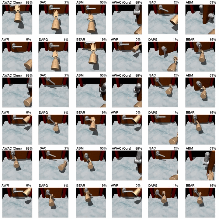
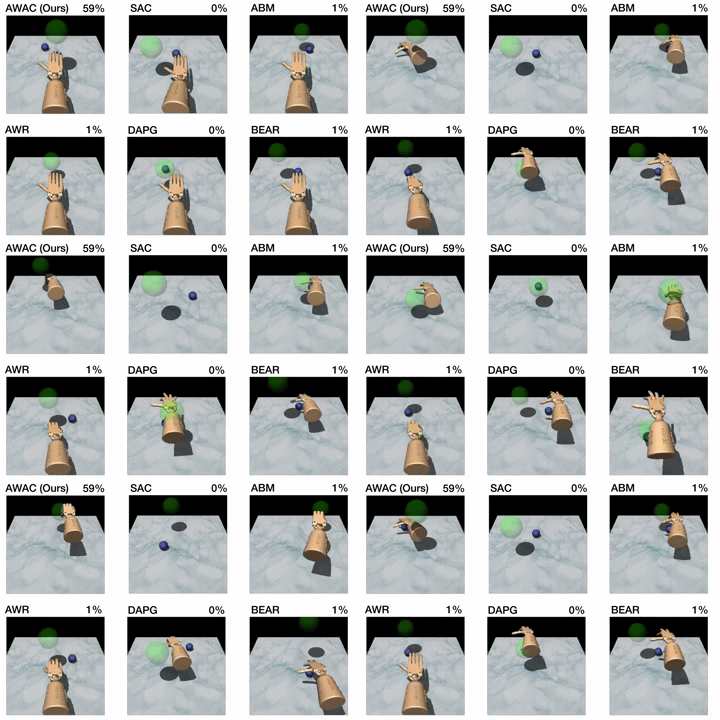
Figure 5. Top: performance shown for various methods after online training (pen: 200K steps, door: 300K steps, relocate: 5M steps). Bottom: learning curves on dextrous manipulation tasks with sparse rewards are shown. Step 0 corresponds to the start of online training after offline pre-training.

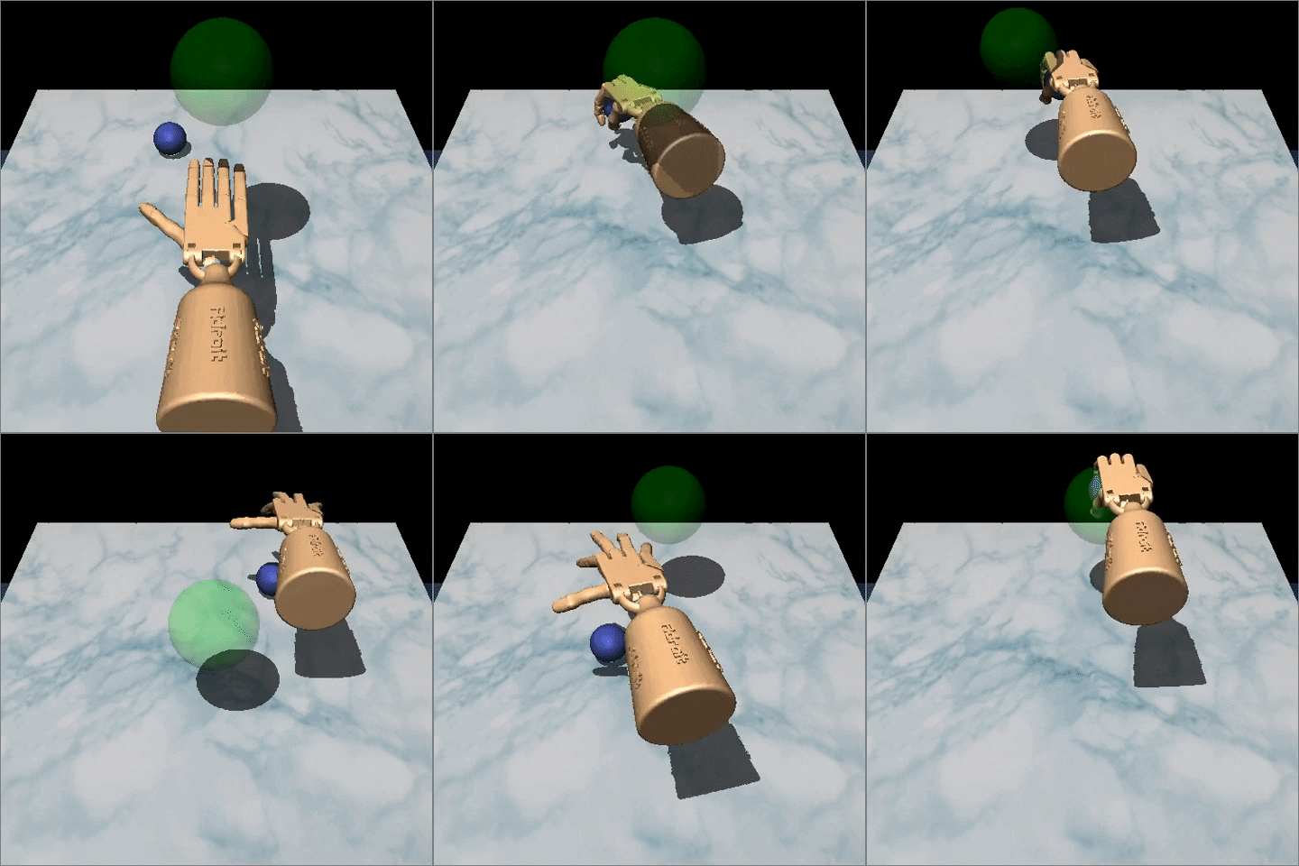
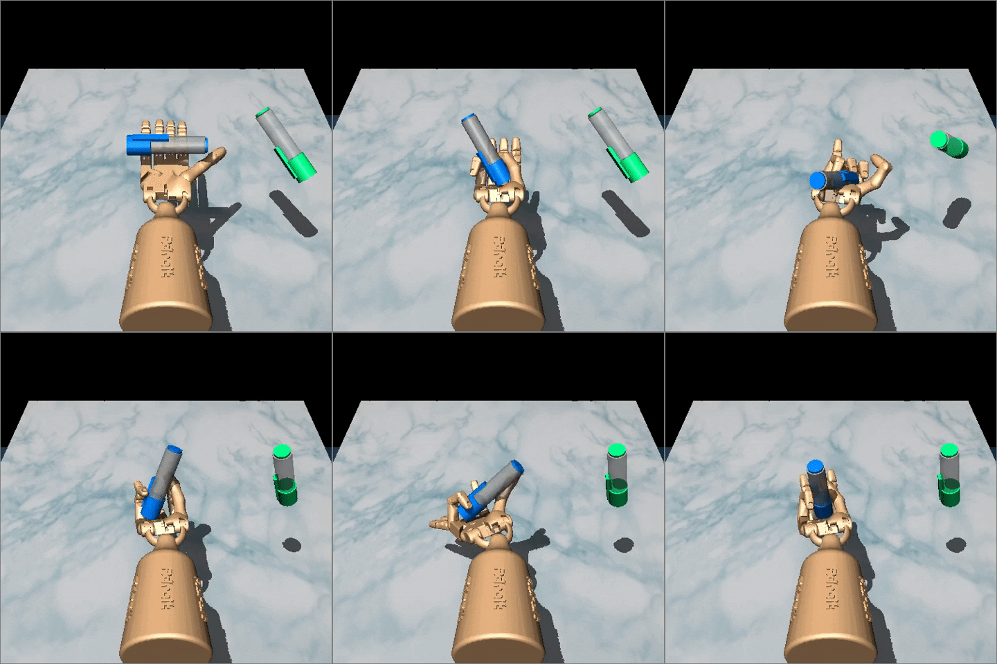
We aim to study tasks representative of the difficulties of real-world robot learning, where offline learning and online fine-tuning are most relevant. One such setting is the suite of dexterous manipulation tasks proposed by Rajeswaran et al., 2017. These tasks involve complex manipulation skills using a 28-DoF five-fingered hand in the MuJoCo simulator: in-hand rotation of a pen, opening a door by unlatching the handle, and picking up a sphere and relocating it to a target location. These environments exhibit many challenges: high dimensional action spaces, complex manipulation physics with many intermittent contacts, and randomized hand and object positions. The reward functions in these environments are binary 0-1 rewards for task completion. Rajeswaran et al. provide 25 human demonstrations for each task, which are not fully optimal but do solve the task. Since this dataset is very small, we generated another 500 trajectories of interaction data by constructing a behavioral cloned policy, and then sampling from this policy.

First, we compare our method on the dexterous manipulation tasks described earlier against prior methods for off-policy learning, offline learning, and bootstrapping from demonstrations. The results are shown in the figure above. Our method uses the prior data to quickly attain good performance, and the efficient off-policy actor-critic component of our approach fine-tunes much quicker than DAPG. For example, our method solves the pen task in 120K timesteps, the equivalent of just 20 minutes of online interaction. While the baseline comparisons and ablations are able to make some amount of progress on the pen task, alternative off-policy RL and offline RL algorithms are largely unable to solve the door and relocate task in the time-frame considered. We find that the design decisions to use off-policy critic estimation allow AWAC to significantly outperform AWR while the implicit behavior modeling allows AWAC to significantly outperform ABM, although ABM does make some progress.

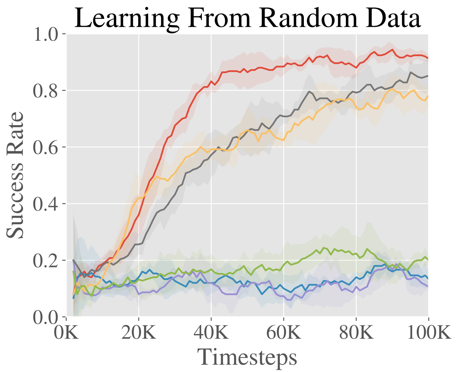
Fine-Tuning from Random Policy Data

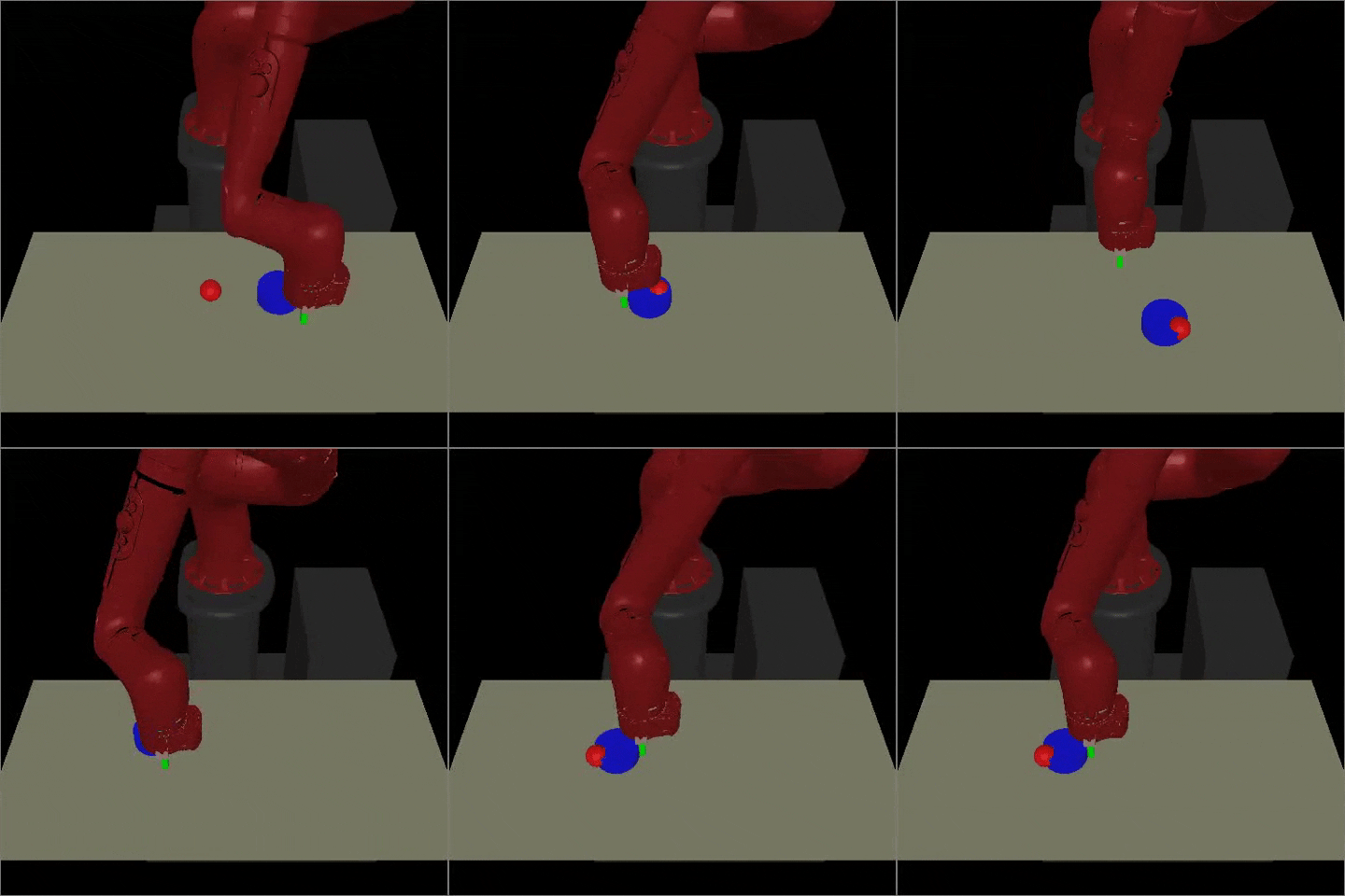
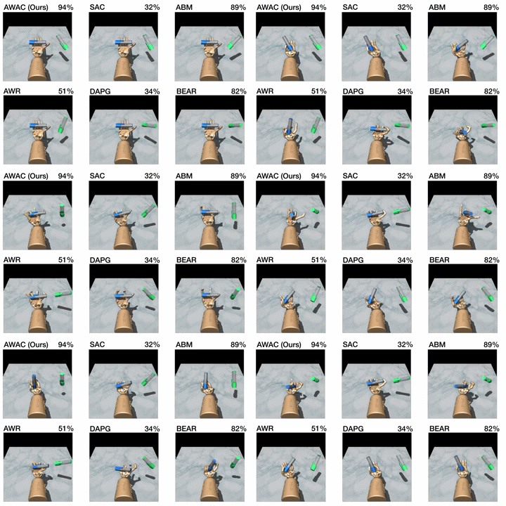
An advantage of using off-policy RL for reinforcement learning is that we can also incorporate suboptimal data, rather than only demonstrations. In this experiment, we evaluate on a simulated tabletop pushing environment with a Sawyer robot.

To study the potential to learn from suboptimal data, we use an off-policy dataset of 500 trajectories generated by a random process. The task is to push an object to a target location in a 40cm x 20cm goal space.

The results are shown in the figure to the right. We see that while many methods begin at the same initial performance, AWAC learns the fastest online and is actually able to make use of the offline dataset effectively as opposed to some methods which are completely unable to learn.

Future Directions

Being able to use prior data and fine-tune quickly on new problems opens up many new avenues of research. We are most excited about using AWAC to move from the single-task regime in RL to the multi-task regime, with data sharing and generalization between tasks. The strength of deep learning has been its ability to generalize in open-world settings, which we have already seen transform the fields of computer vision and natural language processing. To achieve the same type of generalization in robotics, we will need RL algorithms that take advantage of vast amounts of prior data. But one key distinction in robotics is that collecting high-quality data for a task is very difficult - often as difficult as solving the task itself. This is opposed to, for instance computer vision, where humans can label the data. Thus, the active data collection (online learning) will be an important piece of the puzzle.

This work also suggests a number of algorithmic directions to move forward. Note that in this work we focused on mismatched action distributions between the policy $\pi$ and the behavior data $\pi_\beta$. When doing off-policy learning, there is also a mismatched marginal state distribution between the two. Intuitively, consider a problem with two solutions A and B, with B being a higher return solution and off-policy data demonstrating solution A provided. Even if the robot discovers solution B during online exploration, the off-policy data still consists of mostly data from path A. Thus the Q-function and policy updates are computed over states encountered while traversing path A even though it will not encounter these states when executing the optimal policy. This problem has been studied previously. Accounting for both types of distribution mismatch will likely result in better RL algorithms.

Finally, we are already using AWAC as a tool to speed up our research. When we set out to solve a task, we do not usually try to solve it from scratch with RL. First, we may teleoperate the robot to confirm the task is solvable; then we might run some hard-coded policy or behavioral cloning experiments to see if simple methods can already solve it. With AWAC, we can save all of the data in these experiments, as well as other experimental data such as when hyperparameter sweeping an RL algorithm, and use it as prior data for RL.


A preprint of the work this blog post is based on is available here. Code is now included in rlkit. The code documentation also contains links to the data and environments we used. The project website is available here.


from The Berkeley Artificial Intelligence Research Blog https://ift.tt/2DJj3fR
via A.I .Kung Fu
Saturday, August 15, 2020

AI Will Change the World. Who Will Change AI? We Will.


Editor’s Note: The following blog is a special guest post by a recent graduate of Berkeley BAIR’s AI4ALL summer program for high school students.

AI4ALL is a nonprofit dedicated to increasing diversity and inclusion in AI education, research, development, and policy.

The idea for AI4ALL began in early 2015 with Prof. Olga Russakovsky, then a Stanford University Ph.D. student, AI researcher Prof. Fei-Fei Li, and Rick Sommer – Executive Director of Stanford Pre-Collegiate Studies. They founded SAILORS as a summer outreach program for high school girls to learn about human-centered AI, which later became AI4ALL. In 2016, Prof. Anca Dragan started the Berkeley/BAIR AI4ALL camp, geared towards high school students from underserved communities.

Before I Started the Program

When I discovered AI4ALL during the spring semester, I was curious to learn more. I knew that AI had the potential to change everything and that it was something I’d love to be a part of. To prepare for the program, I read up on the BAIR faculty and checked out the BAIR student profiles. I watched Stuart Russell’s TED talk “3 principles for creating safer AI.” The people were all so highly accomplished. And their ideas seemed either super technical, or at the other end of the spectrum, they sounded more like topics from the philosophy department than the EECS department. I realized I had no idea what to expect but decided just to give it a try and get started.

The First Day

After logging into my first day of AI4ALL on Zoom, I was pleasantly surprised by the number of eager and welcoming faces. Among them were Tim Hurt, Eva Chao, Rachel Walsh, Ben Frazier, and Maya Maliviya. They were all there to help us feel comfortable and succeed!

We started off with a quick ice-breaker introduction activity. This particularly resonated with me because it wasn’t like the typical type you’d have on the first day of school. Instead, we were divided into virtual breakout rooms and asked to find as many similarities among our peers as possible. The program was already off to a great start! Within just a few minutes, I learned that five other people in the room have a sibling, have taken chemistry, like pizza, and had a quarantine haircut just like me! It was a great way to encourage collaboration and bonding.

Next, we were joined by BAIR lab professor Anca Dragan for a talk about AI. The presentation was hard to forget because of her passion, her curiosity, and the depth of her knowledge. Anca kickstarted the talk by explaining some examples of AI in real life. This was already so useful because it immediately cleared up the misconceptions about AI. In addition, it allowed everyone to have common, shared learning and not feel excluded if they didn’t know as much about AI before starting the program.

Another element of Anca’s presentation that stood out was her description of an AI game. The game is simple: a robot is positioned in a grid and gains points for reaching gems and loses points for falling in fire pits. Anca walked us through the AI “backstory” of the game. The robot’s goal is to maximize the points earned. As the game’s allotted time decreases, the robot takes less cautious paths (ex: avoiding fire pits) and places its primary focus on gaining points. We learned that this idea of optimization is a core part of all AI systems.

By the end of the day, we were immersed in a Python notebook while conversing with peers in a Breakout Room. AI4ALL equipped us with Python notebooks through Google Colab so we would all be on the same page when talking about code. I really enjoyed this part of the program because it was open-ended and the material was presented in such a clean and convenient fashion. As I read through the content and completed the coding exercises, I couldn’t help but also notice the amusing GIFs embedded here and there! What a memorable way to begin learning AI!

Midway Through the Program

Early on Day 3 of the 4 day AI4ALL program, I began to really understand the significance of AI. Through the eye-opening lecture presentations and discussions, I realized that AI really is everywhere! It’s in our YouTube recommendations, Spotify algorithms, Google Maps, and robotic surgery equipment. That range of applications is part of what makes AI so promising. AI really can be for everyone, whether you’re a developer or a user — it’s not limited to people with mad coding skills. Once I got acquainted with the basics of the subject, I began to see how almost any idea can be reshaped with AI.

I also learned that AI is often different from the way it’s presented in the media. Almost everyone is familiar with the idea of robots taking over jobs, but that isn’t necessarily what will happen. AI still has a long way to go before it will truly “take over the world,” as hypothesized. AI is a work in progress. Like its creators, it has biases. It can unintentionally discriminate. It has adversaries and struggles to find insights with incomplete data. Still, AI has the power to change basic aspects of our world. This is why it is so important to have people from as many backgrounds as possible involved in AI. Introducing people from many different backgrounds into the field allows for a better range of ideas and can help reduce the number of missed “red flags” that might later have a big impact on the lives of real people.

By the End of the Program…

The last two days of AI4ALL sped by in a blur. I couldn’t help but notice how well the program was organized. There was a balanced combination of lectures, discussion, and individual work time for coding and collaborating. I also loved how the content at the end of the program reinforced the content from the start. That aspect of the program’s structure made it so much easier to ask questions, remember ideas, and apply to future activities.

I particularly saw this idea of reinforcement demonstrated in Professor Kamalika Chaduri’s presentation about AI adversaries. She explained how AI algorithms could be manipulated so that an image correctly identified with 50% confidence as a panda would then identify the same image with 90% confidence as a gibbon. On the previous day, Professor Jacob Steinhardt explained how images that appeared similar to the human eye can be tweaked to disrupt AI’s algorithm. In another example, Kamalika described how image pixels could be stored as training data in the form of vectors. This idea built off of Tim Hurt’s earlier point that training data is a result of an input being translated into computer language (e.g. a vector $x$), and then mapped to a label output ($y$).

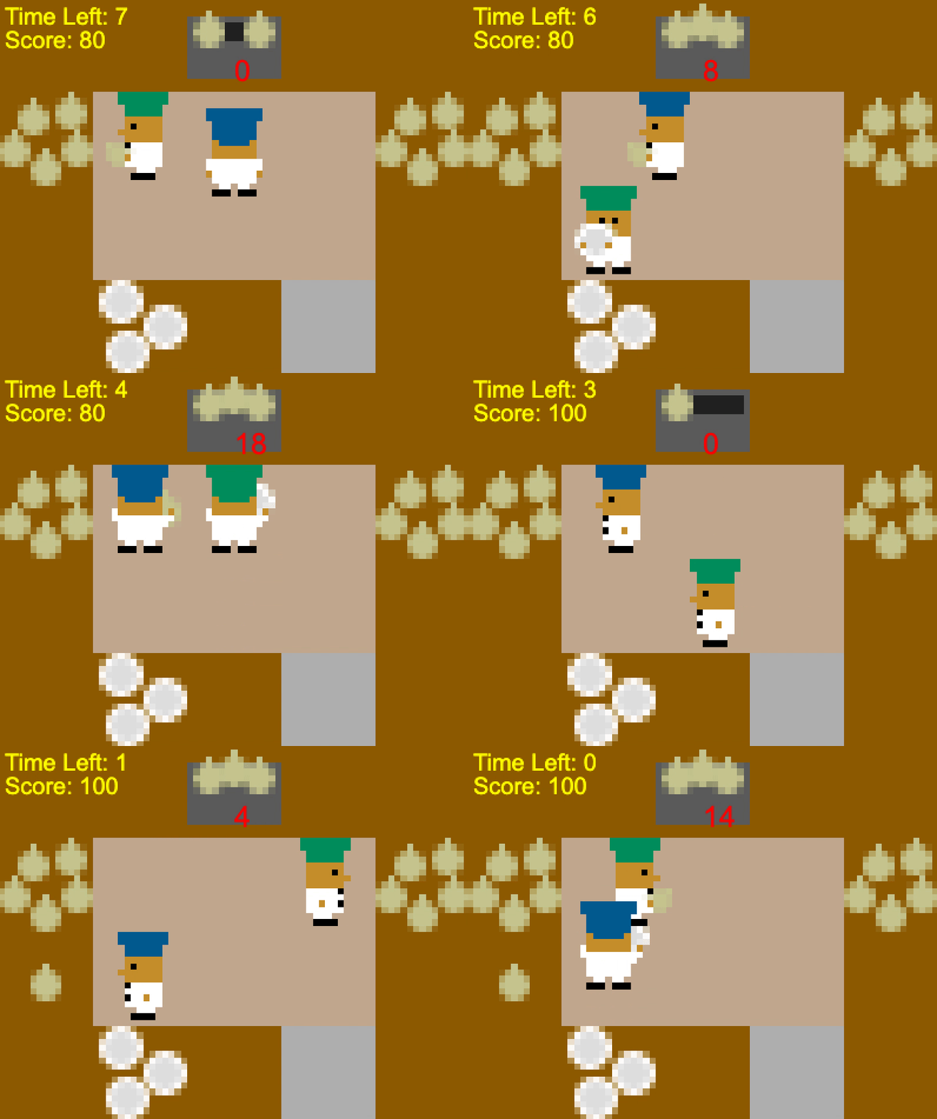
After most of the lectures were done, we began working on our group projects. We were divided into five groups, with each group under the instruction of a Berkeley Ph.D. student. I chose to be in the “Overcooked” group, which was with first-year EECS student Micah Carroll. Micah walked us through the game he’s been using in his research, called Overcooked-AI. Simply put, Overcooked-AI is all about getting the most number of onion soups delivered while cooking in a cramped kitchen.

Once again, we used Colab Notebooks to learn and experiment with the game’s code. Micah patiently took us through the basics of imitation learning, reinforcement learning, decision trees, and graph fitting/displays. He was so open to questions and never hesitated to help! The hours we spent together breezed by, and soon enough I found myself crafting up a final presentation recapping all that I learned. Time really passes when you’re enjoying and learning.

Final Thoughts

In less than a week, the AI4ALL program has shaped my view of AI and my learning process. The lectures, advice panels, and project groups came together to make an unforgettable experience. Beyond learning what AI is and how it works, I now realize that everyone has the potential to explore AI. All you have to do is start. And so, the next time you hear someone say “AI will change the world, but who will change AI?”, you can say with confidence “we will!”

Thank you so much to everyone who made AI4ALL possible!


from The Berkeley Artificial Intelligence Research Blog https://ift.tt/3g7CnAQ
via A.I .Kung Fu

Monday, August 3, 2020

Estimating the fatality rate is difficult but doable with better data

The case fatality rate quantifies how dangerous COVID-19 is, and how risk of death varies with strata like geography, age, and race. Current estimates of the COVID-19 case fatality rate (CFR) are biased for dozens of reasons, from under-testing of asymptomatic cases to government misreporting. We provide a careful and comprehensive overview of these biases and show how statistical thinking and modeling can combat such problems. Most importantly, data quality is key to unbiased CFR estimation. We show that a relatively small dataset collected via careful contact tracing would enable simple and potentially more accurate CFR estimation.

What is the case fatality rate, and why do we need to estimate it?

The case fatality rate (CFR) is the proportion of fatal COVID-19 cases. The term is ambiguous, since its value depends on the definition of a ‘case.’ No perfect definition of the case fatality rate exists, but in this article, I define it loosely as the proportion of deaths among all COVID-19-infected individuals.

The CFR is a measure of disease severity. Furthermore, the relative CFR (the ratio of CFRs between two subpopulations) enables data-driven resource-allocation by quantifying relative risk. In other words, the CFR tells us how drastic our response needs to be; the relative CFR helps us allocate scarce resources to populations that have a higher risk of death.

Although the CFR is defined as the number of fatal infections, we can not expect that dividing the number of deaths by the number of cases will give us a good estimate of the CFR. The problem is that both the numerator (#deaths) and the denominator (#infections) of this fraction are uncertain for systematic reasons due to the way data is collected. For this reason, we call that estimator “the naive estimator”, or simply deaths/cases, and denote it as $E_{\rm naive}$.

Why are (all) CFR estimates biased?

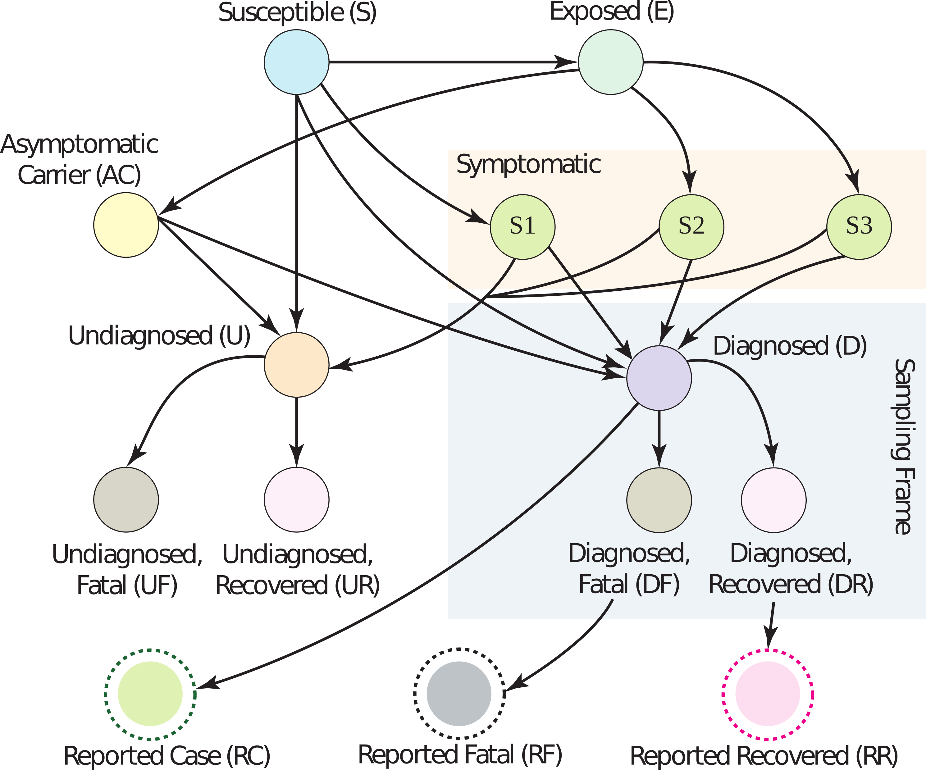
Graphical model.
Fig. 1 Dozens of biases can corrupt the estimation of the CFR. Surveillance data gives partial information within the ‘sampling frame’ (light blue rectangle). Edges on the graph correspond roughly to conditional probabilities; e.g., the edge from D to DF is the probability a person dies if they are diagnosed with COVID-19.

In short, all CFR estimates are biased because the publicly available data is biased. We have reasson to believe that we are losing at least 99.8% of our sample efficiency due to this bias. There is a “butterfly effect” caused by non-random sampling: a tiny correlation between the sampling method and the quantity of interest can have huge, destructive effects on an estimator. Even assuming a tiny 0.005 correlation between the population we test and the population infected, testing 10,000 people for SARS-CoV-2 is equivalent to testing 20 individuals randomly. For estimating the fatality rate, the situation is even worse, since we have ample evidence that severe cases are preferentially diagnosed and reported. In the words of Xiao-Li Meng, “compensating for [data] quality with quantity is a doomed game.” In our HDSR article, we show that in order for the naive estimator $E_{\rm naive}$ to converge to the correct CFR, there must be no correlation between fatality and being tested — but severe cases are much more likely to be tested. Government and health organizations have been explicitly reserving tests for severe cases due to shortages, and severe cases are likely to go to the hospital and get tested, while asymptomatic ones are not.

The primary source of COVID-19 data is population surveillance: county-level aggregate statistics reported by medical providers who diagnose patients on-site. Usually, somebody feels sick and goes to a hospital, where they get tested and diagnosed. The hospital reports the number of cases, deaths, and sometimes recoveries to local authorities, who release the data on a weekly basis. In reality, there are many differences in data collection between nations, local governments, and even hospitals.

Dozens of biases are induced by this method of surveillance, falling coarsely into five categories: under-ascertainment of mild cases, time lags, interventions, group characteristics (e.g. age, sex, race), and imperfect reporting and attribution. An extensive (but not exhaustive) discussion of the magnitude and direction of these biases is in Section 2 of our article. Without mincing words, current data is extremely low quality. The vast majority of people who get COVID-19 go undiagnosed, there are misattributions of symptoms and deaths, data reported by governments is often (and perhaps purposefully) incorrect, cases are defined inconsistently across countries, and there are many time-lags. (For example, cases are counted as ‘diagnosed’ before they are ‘fatal’, leading to a downward bias in the CFR if the number of cases is growing over time.) Figure 1 has a graphical model describing these many relationships; look to the paper for a detailed explanation of what biases occur across each edge.

Correcting for biases is sometimes possible using outside data sources, but can result in a worse estimator overall due to partial bias cancellation. This is easier to see through example than it is to explain. Assume the true CFR is some value $p$ in the range 0 to 1 (i.e., deaths/infections is equal to $p$). Then, assume that because of under-ascertainment of mild cases, there are too many fatal cases being reported, which means $E_{\rm naive}$ converges to $bp > p$ (in other words, it is higher than it should be by a factor of $b$). Also assume the time-lag between diagnosis and death causes the proportion of deaths to diagnoses to decrease by the same factor $b$. Then, $E_{\rm naive}$ converges to $b(p/b)=p$, the correct value. So, even though it might seem to be an objectively good idea to correct for time-lag between diagnosis and death, it would actually result in a worse estimator in this case, since time-lag is helping us out by cancelling out under-ascertainment.

The mathematical form of the naive estimator $E_{\rm naive}$ allows us to see easily what we need to do to make it unbiased. With $p$ being the true CFR, $q$ being the reporting rate, and $r$ being the covariance between death and diagnosis, the mean of $E_{\rm naive}$ is:

This equation is pretty easy to understand. We wanted $\mu$ to be equal to $p$. Instead, we got an expression that depends on $r$, $q$, and $N$. The $r/q$ term is the price we pay if people who are diagnosed are more likely to eventually die. We want $r/q=0$, but in practice, $r/q$ is probably much larger than $p$. (Actually, if we assume the CFR is around 0.5% and the measured CFR is 5.2% on June 22, 2020, then $r/q \ge 0.047 \gg 0.005$.) In other words, $r/q$ is the bias, and it can be large. The term $p$ is the true CFR, which we want. And the factor $(1−(1−q)^N)$ is what we pay because of non-response; however, it’s not a big deal, because it disappears quite fast as the number of samples $N$ grows. So really, our primary concern should be achieving $r=0$, because — and I cannot stress this enough — $r/q$ does not decrease with more samples; it only decreases with higher quality samples.

What are strategies for fixing the bias?

In our article, we outline a testing procedure that helps fix some of the above dataset biases. If we collect data properly, even the naive estimator $E_{\rm naive}$ has good performance.

In particular, data should be collected via a procedure like the following:

  1. Diagnose person $P$ with COVID-19 by any means, like at a hospital.

  2. Reach out to contacts of $P$. If a contact has no symptoms, ask them to commit to getting a COVID-19 test.

  3. Test committed contacts after the virus has incubated.

  4. Keep data with maximum granularity while respecting ethics/law.

  5. Follow up after a few weeks to ascertain the severity of symptoms.

  6. For committed contacts who didn’t get tested, call and note if they are asymptomatic.

This protocol is meant to decrease the covariance between fatality and diagnosis. If patients commit to testing before they develop symptoms, this covariance simply cannot exist. However, there may still be issues with people dropping out of the study; if this is a problem in practice, it can be mitigated by a combination of incentives (payments) and consistent follow-ups.

A figure.
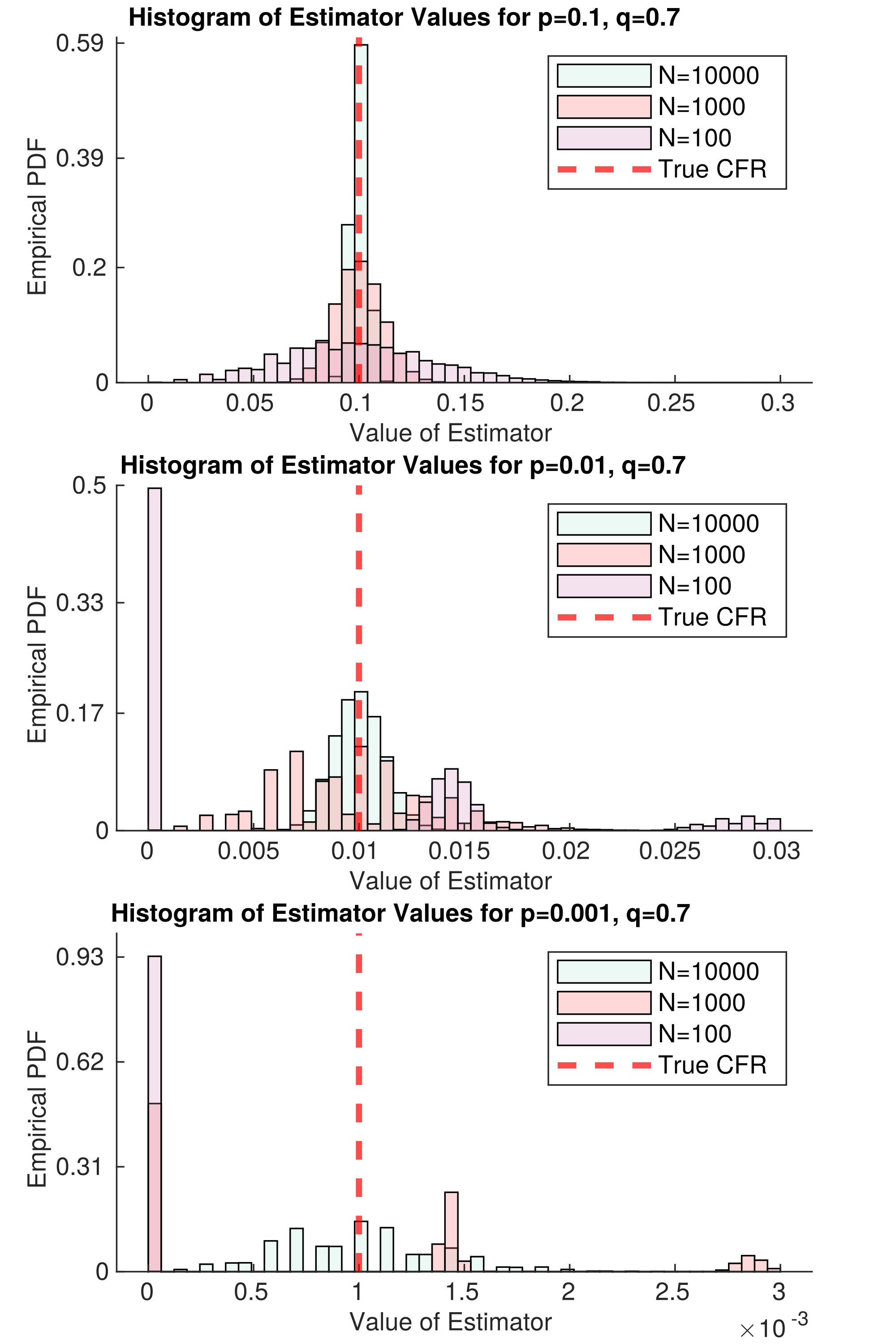
Fig. 2 Assuming data collection induces no correlation between disease severity and diagnosis, as the true CFR decreases, it requires more samples to estimate. The variable p is the true CFR, and q is the response rate. Each histogram represents the probability the naive estimator will take on a certain value, given N samples of data (different colors correspond to different values of N). The three stacked plots correspond to different values of p; the smaller p is, the harder it is to estimate, since death becomes an extremely rare event.

Figure 2 represents an idealized version of this study. In the best case scenario, there is no covariance between death and diagnosis. Then, we only need $N=66$ samples for our estimator of the CFR to be approximately unbiased, even if $p=0.001$ ($1/1000$ cases die). Problems remain in the case that $p$ is small; namely, death is so rare that we need tons of samples to decrease the variance of our estimator. This will require lots of samples. But even if no deaths are observed, we get a lot of information about $p$; for example, if $N=1000$ and we have not observed a single death, then we can confidently say that $p<0.01$ within the population we are sampling. This is simply because in the second panel of Figure 2, there is nearly zero mass in the $N=1000$ histogram at $E_{\rm naive} = 0$. With this in mind, we could find the largest possible p that is consistent with our data — this would be a conservative upper bound on $p$, but it would be much closer to the true value than we can get with current data.

This strategy mostly resolves what we believe is the largest set of biases in CFR estimation — under-ascertainment of mild cases and time-lags. However, there will still be lots of room for improvement, like understanding the dependency of CFR on age, sex, and race. (In other words, the CFR is a random quantity itself, depending on the population being sampled.) Distinctions between CFRs of these strata may be quite small, requiring a lot of high-quality data to analyze. If $p$ is extremely low, like 0.001, this may require collecting $N=100,000$ or $N=1,000,000$ samples per group. Perhaps there are ways to lower that number by pooling samples. Even though making correct inferences will require careful thought (as always), this data collection strategy will make it much simpler.

I’d like to re-emphasize a point here: collecting data as above will make the naive estimator $E_{\rm naive}$ unbiased for the sampled population. But the sampled population may not be the population we care about. However, there is a set of statistical techniques collectively called ‘post-stratification’ that can help deal with this problem effectively — see Mr. P.

If you read our academic article, we provide some thoughts on how to use time-series data and outside information to correct time-lags and relative reporting rates. Our work was very heavily based on one of Nick Reich’s papers. However, as I claimed earlier, even fancy estimators cannot overcome fundamental problems with data collection. I’ll defer discussion of that estimator, and the results we got from it, to the article. I’d love to hear your thoughts on it.

CFR estimation is clearly a difficult problem — but with proper data collection and estimation guided by data scientists, I still believe that we can get a useful CFR estimate. This will help guide public policy decisions about this urgent and ongoing pandemic.


This blog post is based on the following paper:


from The Berkeley Artificial Intelligence Research Blog https://ift.tt/3i72v03
via A.I .Kung Fu